Simulation Study of Adaline Neural Network Stochastic LMS Algorithm
1 Introduction One of the most important functions of artificial neural networks is classification. For linearly separable problems, a single neuron using a hard limiting function can be successfully classified by a simple learning algorithm. That is, for input vectors in two different classes, the output value of the neuron is 0 or 1. But for most non-linear classifiable, hard-limiting neurons can not complete the classification function. The adaptive linear element Adaline (Adap-TIve LiIlear Element) is a kind of deduction element with linear function function. It can be realized under the statistical significance of the least square LMS (Least Mean Square) of the actual output and the ideal expected value. The classification of the best nonlinear separable set, that is, according to the statistical significance of the least squares, the mean square value of the error between the actual output value and the ideal expected value is the smallest. The algorithm that can achieve this purpose is called least squares. Learning algorithm or LMS algorithm.
2 Adaline's LMS algorithm principle Suppose the input vector X = [x1, x2, ..., xn] and the weighted vector W = [ω1, ω2, ..., ωn], then the output of the neuron is:
Definition ε (k) is the error between the ideal output value d (k) and the actual output value y (k), ie ε (k) = d (k) -y (k), and its mean square value is recorded as E [ ε2 (k)], let ζ (k) = E [ε2 (k)], then: ![]()
From equation (2), we know that there must be an optimal weighting vector W * to minimize ζ (k). At this time, the gradient of ζ (k) relative to W is equal to zero, so that we can obtain:

Although formula (3) gives a method to find the best weighted vector, it requires a lot of statistical calculations, and when the dimension of the input vector X is large, it is necessary to solve the inverse problem of the higher-order matrix. These are all mathematical calculations. It is very difficult.
3 Stochastic approximation LMS learning algorithm is proposed In order to solve the problems in equation (3), some scholars have proposed a strict recursive algorithm and a random approximation algorithm for LMS learning problems. Here, the algorithm principle is briefly described. The strict recursive algorithm of the LMS learning problem is to adjust W for each time series variable k when the initial weight vector W (0) is arbitrarily set:
![]()
In this way, we can guarantee a strict optimal solution and avoid matrix inversion. But each step of the learning process still requires a lot of statistical calculations, and the statistical calculation difficulties still need to be solved.
The random approximation algorithm of the LMS learning problem corrects the weight adjustment formula to the following form:

The difference between this method and the previous algorithm is that: replace E [ε (k) X (k)] with ε (k) X (k), so as to avoid the difficulty of statistical calculation, but at the same time make the changes of the weighting vector tend to be random; The amplitude α becomes an amount that changes with time sequence k. It can be proved that learning is convergent when α (k) satisfies the following conditions: α (k) is the time sequence k∞ ∞
Non-increasing function of ![]() Under the condition that k = 0 k = 0, the probability that W (k) tends to W * as k increases is 1.
Under the condition that k = 0 k = 0, the probability that W (k) tends to W * as k increases is 1.
4 Random approximation LMS algorithm simulation Follow the steps below to simulate the random approximation algorithm programming:
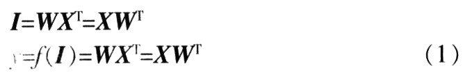
(1) The sine wave and triangle wave shown in Fig. 1 are respectively sampled at 64 points to form a 64-dimensional input sample vector.
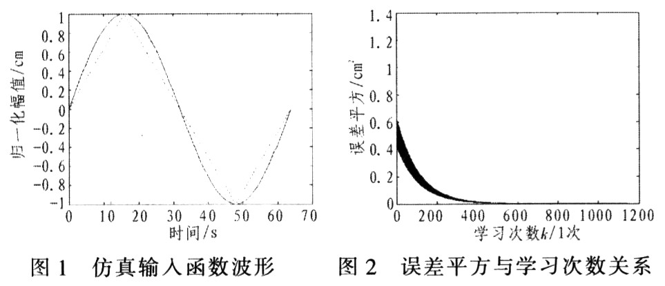
(2) W (0) selects a random vector that is uniformly distributed between (0, 1), the initial step parameter α is selected as 0.03, and the squared critical value of the error ε02 (k) = 10-5 is selected. X0, X1 are fed into neurons using linear function alternately and repeatedly, and training is repeated until ε2 (k) ≤ε02 (k), so that the relationship between the error square and the number of learning times can be obtained, as shown in Figure 2.
It can be seen from Figure 2. When α = 0.03, the learning is convergent, the learning frequency k = 1147, and ε (k) = 3.2 × 10⁻³ when the learning is completed, the square of which is smaller than the determined ε02 (k). Send X0 and X1 into the neuron again, and after calculation, the actual output values ​​Y0 = 0.003 9 and Y1 = 0.999 9 are obtained, which is quite close to the expected output value, thus completing the classification of X0 and X1.
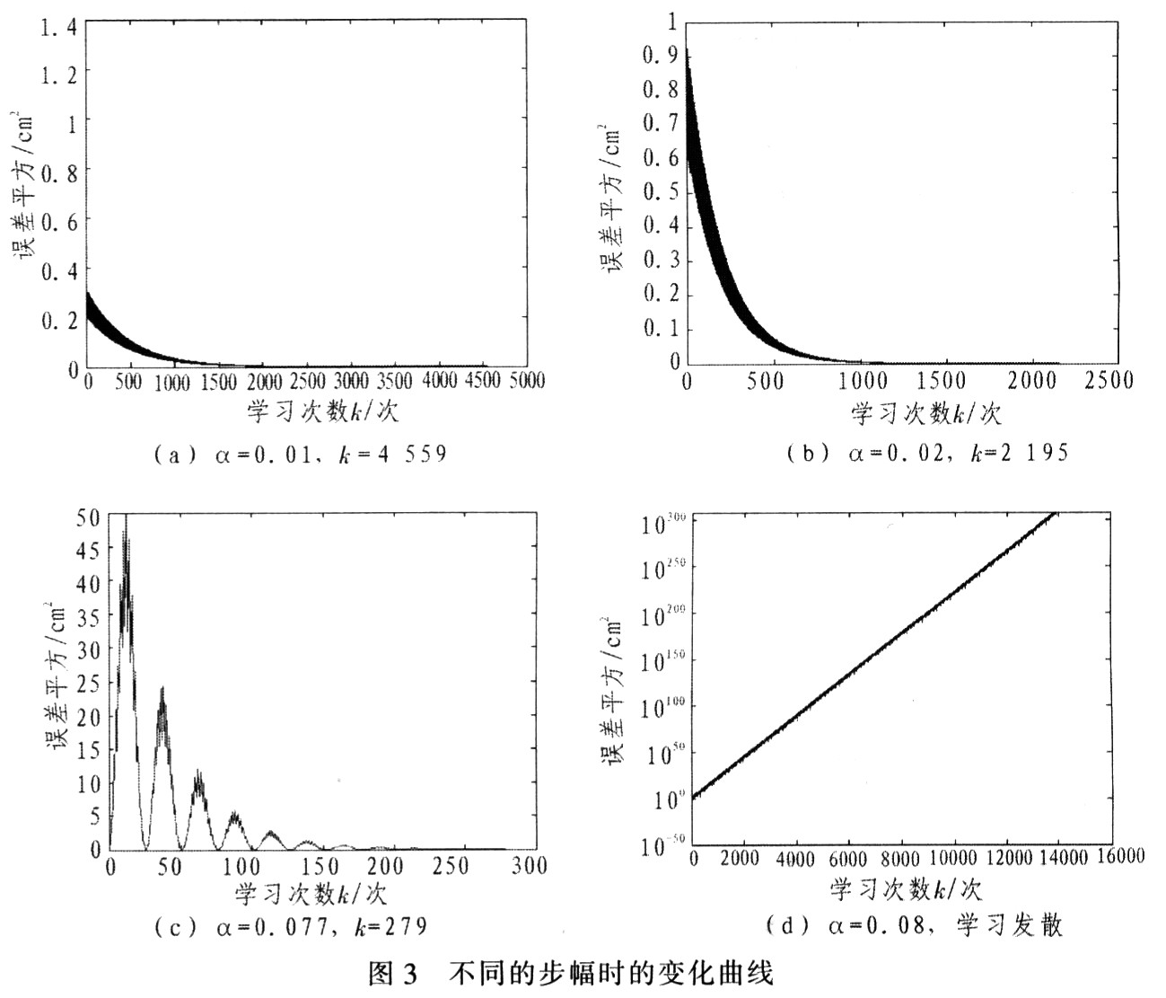
(3) Set different steps α, calculate and draw the change curve of ε2 (k) respectively, and observe the relationship between ε2 (k) convergence, convergence speed and α. The test results are shown in Figure 3. It can be seen from Figure 3 that when α is small, the learning converges, the learning speed is very slow, and the stability of the convergence is good; when α increases, the learning still maintains convergence, but the learning speed is accelerated and the stability is reduced; when When α = 0.08, learning no longer converges.
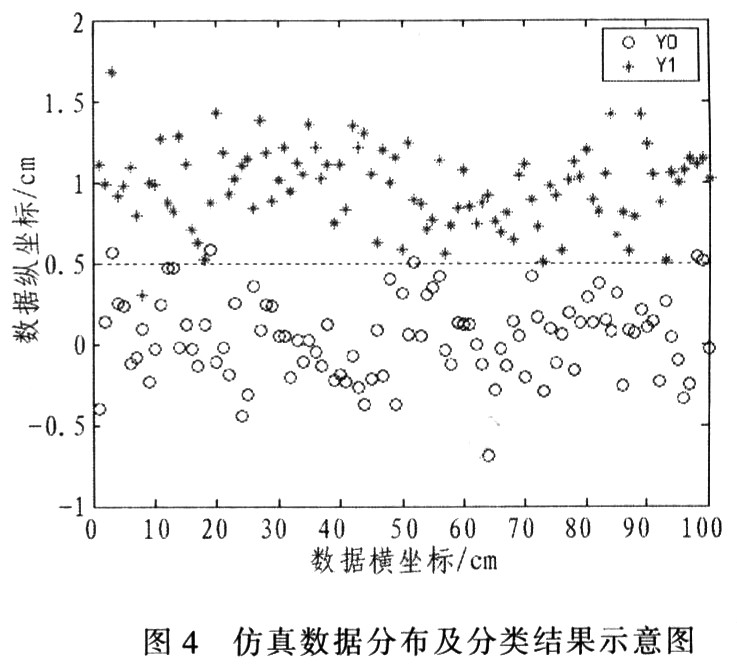
(4) Simulation accuracy and noise resistance. A series of noisy sine waves and triangle waves are generated as input vectors, and the superimposed noise follows a normal distribution N (0, σ2). Specify Pn as the probability of correctly identifying X0, P1 as the probability of correctly identifying X1, and ERR as the number of output errors (total sample: 1 000). Table 1 can be obtained by detection. It can be seen from Table 1 that when the noise variance σ2 is small, the Adaline neuron using the random approximation algorithm can almost recognize the input vector without error; but when the noise variance gradually increases, the probability of misjudgment also increases. Under the condition of learning convergence, the stride α has almost no effect on the accuracy of the neuron output. Figure 4 shows that when the total sample is 200, the fixed α = 0.03. Schematic diagram of the classification results when α2 = 3x10⁻³.
5 Simulation results and analysis First, the two waveforms are sampled at 64 points, and then the random approximation algorithm is used to classify the two waveforms, which is also equivalent to the classification of two points in a 64-dimensional space. The simulation results show that for different initial steps α, the training time of neurons to complete the learning task is different; on the premise of ensuring learning convergence, the larger α, the faster the convergence speed, but the stability of the convergence becomes worse. The initial value of the weight vector W (0) has no effect on the convergence of learning. Finally, the learning results of neurons are tested, and the test results verify the correctness and noise resistance of neuron classification after learning and training. It can be seen from the principle of the network that in the random approximation algorithm, if α (k) is a non-increasing function of time series k, and 
Learning is convergent. However, in this simulation, a constant step value α is used, so that only when the value of α is relatively small, the learning convergence can be guaranteed. In order to improve the algorithm, the time-varying stride α (k) = 1 / pk + q can be used, which not only satisfies the condition of the stride factor convergence, but also ensures that the stride factor is larger at the beginning of learning, and as the learning progresses slowing shrieking.
Rainproof Cummins Diesel Generator
Waterproof Diesel Generator,Rainproof Cummins Diesel Generator,600Kw Cummins Rainproof Generator,600Kw Rainproof Cummins Diesel Generator
Jiangsu Lingyu Generator CO.,LTD , https://www.lygenset.com